Introduction

In this Blog, I will discuss the LSeg (Language-driven Semantic Segmentation) paper. In recent years, semantic segmentation has gained significant traction in computer vision. Incorporating natural language adds another layer of complexity—especially when asking a model to predict unseen classes, a key limitation of traditional architectures. LSeg addresses these exact challenges.

While few-shot learning approaches exist, they still require labeled training samples for new classes. In contrast, the authors focus on zero-shot learning. By leveraging language embeddings, LSeg can identify both seen and unseen classes without additional labeled data. Inspired by CLIP’s strong zero-shot capabilities, the authors adapt this concept to dense prediction tasks.

Main Idea

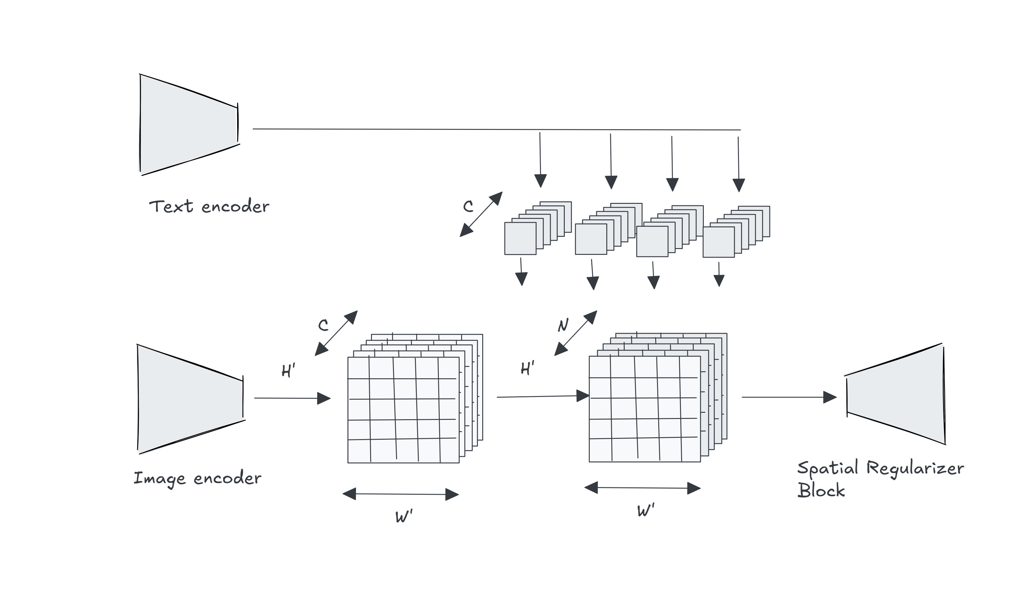
The authors’ core approach is to map both image pixels and text labels into a shared embedding space, allowing the model to assign a semantic label to every single pixel.

Text Encoder:

The text encoder embeds $N$ potential labels into a continuous vector space $R^C$. To accomplish this, the authors utilize CLIP’s pretrained text encoder.

Image Encoder:

Similar to the text encoder, the image encoder generates a dense embedding vector for every pixel. The authors use Dense Prediction Transformers (DPT) for this component. Given an image of size $H \times W$ and a downsampling factor $s$ $$\tilde{H} = \frac{H}{s}, \tilde{W} = \frac{W}{s}$$
the model outputs dense feature embeddings of shape $$I \in R^{\tilde{H} \times \tilde{W} \times C}$$

Word-Pixel Correlation Tensor:

Once the image and text features are embedded, the model computes their correlation using a dot product (or cosine similarity). It will create tensor of size $$\tilde{H} \times \tilde{W} \times N$$ defined as

For N = 1, embedding size of Image $I\_ij$ and Text $T\_K$

Below is the pixelwise softmax

During training, LSeg minimizes the standard spatial cross-entropy loss across all pixels, encouraging the model to align visual pixel representations directly with their corresponding text label embeddings.

Spatial Regularizer Block:

To address memory constraints during training and inference, the authors introduce two spatial-text fusion blocks:

• DepthwiseBlock: Applies depthwise convolutions followed by a non-linear activation to efficiently fuse text and image representations.
• BottleneckBlock: Further enhances the depthwise convolutions by incorporating the output of a max-pooling operation over the set of text labels, capturing the most prominent label interactions.

Finally, a bilinear upsampling block restores the spatial feature maps from $$\frac{H}{s} \times \frac{W}{s}$$ back to the original image dimensions ($H \times W$), yielding high-resolution pixel-level predictions.

My Implementation

Unlike standard zero-shot setups, my objective was supervised remote sensing segmentation using a lightweight foundation model (prithvi_eo_v2_tiny_tl) aligned with a pretrained CLIP text encoder.

Methodology Highlights:

• Decoder Modification: Kept Prithvi’s spatial decoder, removed the default classification head, and added a projection layer to map dense spatial features into the text embedding space. An encoder-only baseline yielded low-resolution, “blobby” segmentations; retaining the decoder restored finer spatial boundary definition.
• Pixel-Text Alignment: Evaluated dot-product similarity between projected spatial features and text embeddings, applying a pixel-wise softmax to derive output class probabilities.
• Fine-Tuning: Trained for ~12 epochs using a 300-image subset of the Prithvi dataset.
• Prompt Engineering: Applied mean centering to neutralize class biases and prompt templating (e.g., “remote sensing view of [class]”) to enrich text feature representations.

Key Improvements Made

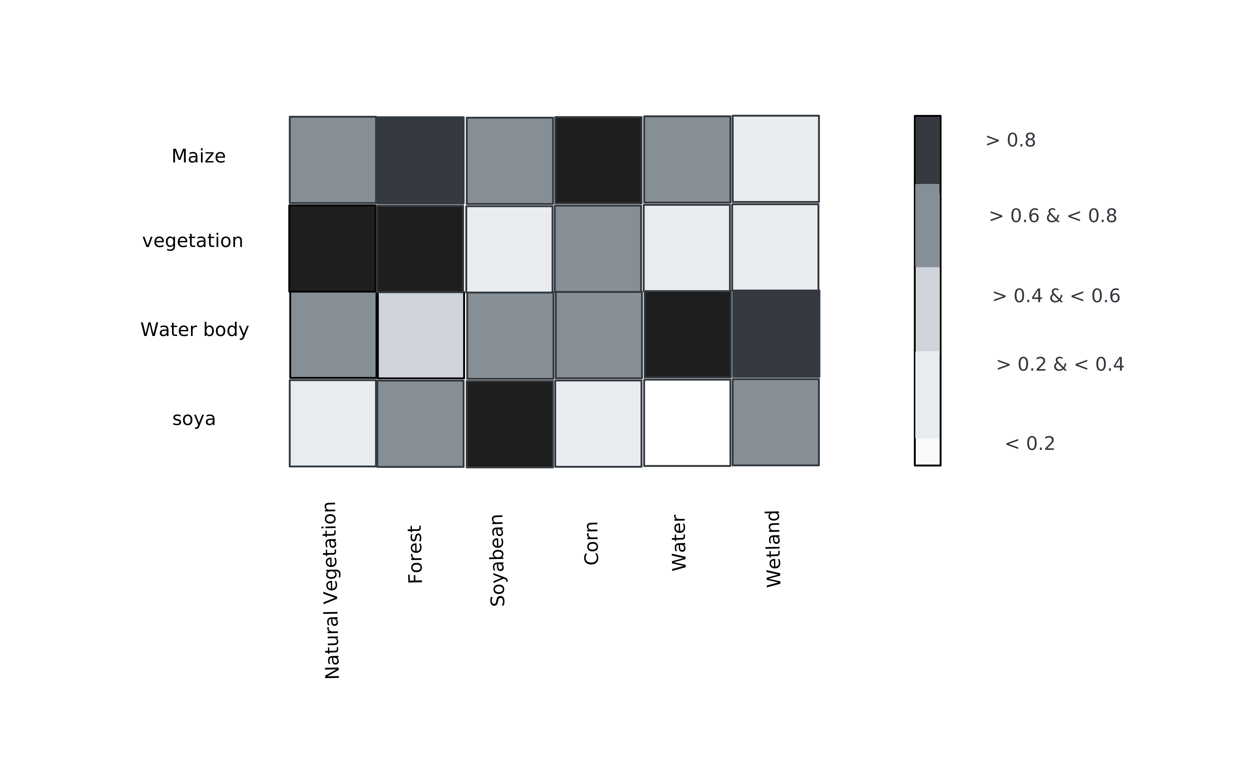
Heatmap matrix showing pre-mean-centering cosine similarity scores between fixed dataset target classes (x-axis) and prompt vocabulary terms (y-axis).

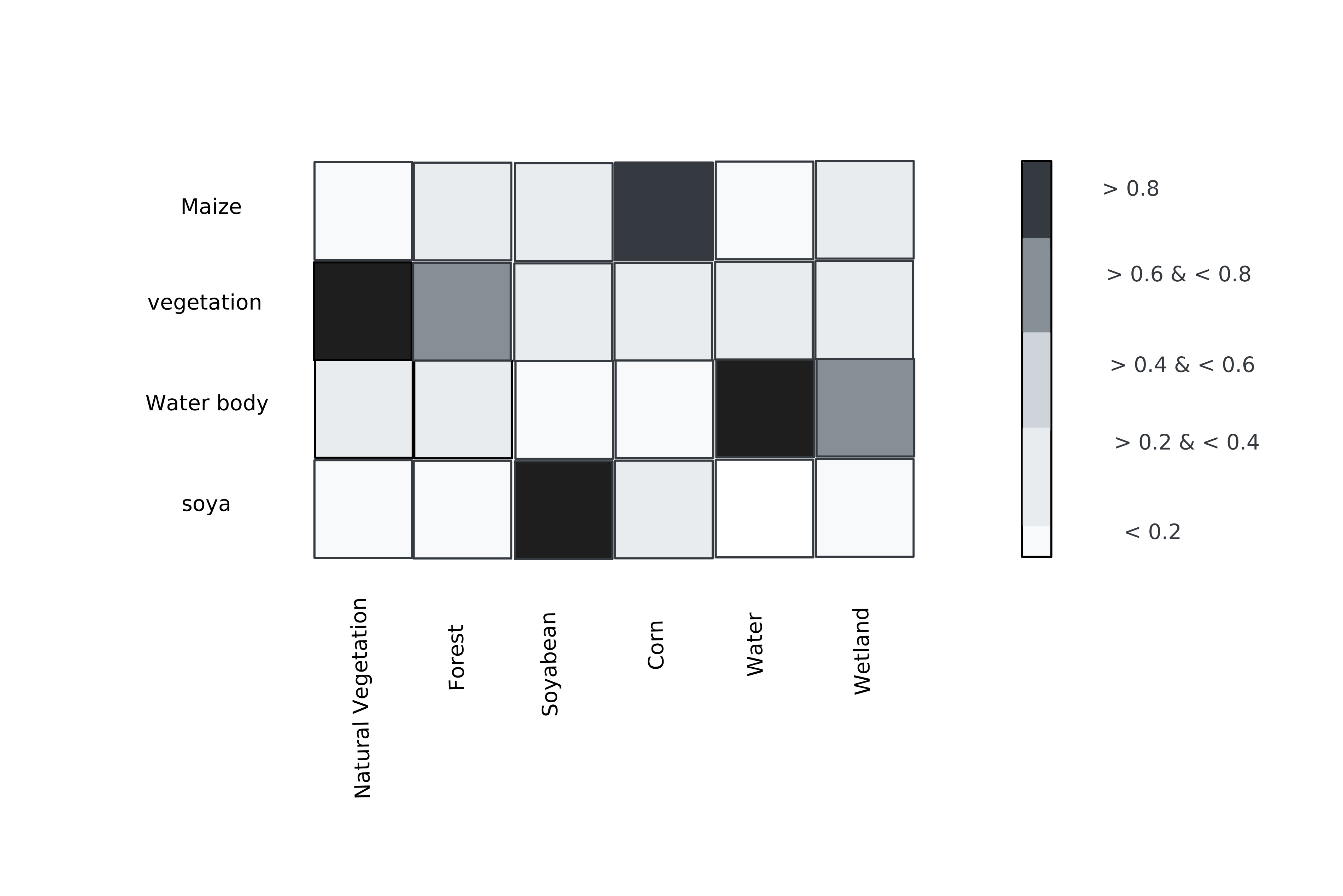
Heatmap matrix showing post-mean-centering cosine similarity scores between fixed dataset target classes (x-axis) and prompt vocabulary terms (y-axis).

Limitation

While LSeg provides an elegant baseline for language-guided segmentation, several practical limitations emerged during experimentation on remote sensing data:

1. Prompt Complexity Ceiling: The text-image correlation mechanism degrades when exposed to lengthy or multi-attribute text prompts. While basic action prompts (e.g., “detect water”) yield clear similarity maps, long-form natural language prompts degrade segmentation precision.
2. Domain-Specific Vocabulary Drift: The model’s performance drops when encountering out-of-vocabulary spatial features. Satellite imagery presents intricate spatial textures, non-standard orientations, and multi-spectral signals that are far more challenging to align with text embeddings than standard RGB natural images.

🔗 Check demo app and code